XXXXXXXXXXXXXXXXXXXXXXXXXXXXXXXXXXXXXXXXXXXXXXXXXXXXXXXXXXXXXXXXXXXXXXXXXXXXXXXXXXXXXXXXXXXXXXXXXXXXXXXXXXXXXXXXXXXXXXXXXXXXXXXXXXXXXXXXXXXXXXXXXXXXXXXX''"> Vibration Fatigue
The techniques described in this section deal with random vibration induced fatigue, which is calculated from
random vibration and/or
frequency response FE analysis results. A
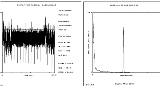
Power Spectral Density Function (PSDF or PSD) is the most common way of representing the loadings or responses in the frequency domain. The transformation between time domain, i.e., the time history of the loading, and the frequency domain, i.e., a PSD, should not trouble the reader. The PSD simply shows the frequency content of the time signal and is an alternative way of specifying the time signal. It is obtained by utilizing the
Fast Fourier Transform (FFT). Figure 14‑1 shows this equivalence for a typical structural response signal.
Transforming from the frequency domain to the time domain is also a relatively easy task which can be done using the Inverse Fourier Transform (IFT). However, when transforming in this direction the random phase angles attributable to each frequency component (which have not been kept when converting to the frequency domain) have to be generated or re-generated. This can be done such that a statistically equivalent signal can be reproduced.
Figure 14‑1 PSDs and the Transformation Between
Time and Frequency Domains
It is not the intention of this manual to teach the user all there is to know about random vibration. For those unfamiliar with random vibration techniques, refer to
Vibration Fatigue Theory (p. 674) in the MSC Fatigue User’s Guide.
Definitions
These are some of the terms you might come across when going through the Vibration Fatigue example:
• Power Spectral Density (PSD)
• Transfer function
• Irregularity factor
• Narrow band
• Wide band
• White noise
• Probability Density Function (PDF)
• Expected mean crossing
• Expected number of peaks
• Spectral movement
All of these terms are defined in Appendix A,
Glossary Terms.
Frequency Domain Life Estimation - General Procedure
This section provides a brief summary of techniques for computing fatigue life, or damage, from a PSD of stress or strain. These fall into two broad categories: those that estimate fatigue life directly and those that compute rainflow cycle PDFs as an intermediate stage. All of the approaches have now been brought together in MSC Fatigue.
General Fatigue Damage Equation
The general Fatigue Damage equation for the Frequency Domain is shown below. P(S) is obtained with the appropriate vibration fatigue modeler instead of with rainflow cycle counting used in the time-based approach. Refer to the
MSC Fatigue 2005 QuickStart Guide MSC Fatigue User’s Guide.
.
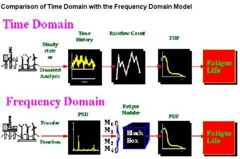
To obtain a time history of stress or strain response, either a steady state or transient analysis would be required. For the random response history indicated this would obviously be a transient analysis. In the frequency domain a transfer function would first be computed for the structural model. This is completely independent of the input loading and is a fundamental characteristic of the system, or model. The PSD response caused by any PSD of input loading is then obtained by multiplying the transfer function by the input loading PSD. Further response PSDs caused by additional PSDs of input loading can then be calculated with a trivial amount of computing time. An essential requirement of a structural analysis in the frequency domain is that it results in a PSD which is equivalent to the time history obtained using the transient approach. The rest of the design process is then concerned with using the vibration fatigue tools to compute fatigue life directly from these PSDs of stress. These tools either estimate rainflow histograms (or PDFs), or fatigue life directly. These are shown schematically in the dashed box in the figure above under the heading fatigue modeler. This is intended to show that the time and frequency domain processes are actually very similar. The only differences being the structural analysis approach used (time or frequency domain) and the fact that a fatigue modeler is required to transform from a PSD of stress to the rainflow cycle histogram. In this context the vibration fatigue modeler can be envisaged as just another form of rainflow cycle counting.
Vibration Model Setup
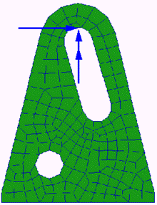
A simple bracket, shown to the left, is subject to random vibration excitations defined by loading power spectral density (PSD) functions, which induce serious fatigue damage around the attachment location (the circular hole). The bracket is subject to three input loads, a vertical and horizontal force and a twisting moment, at the far end of the slot. The model is constrained around the circular hole. A random vibration analysis is performed by combining FE frequency response analysis results using three unit loads combined with the loading input PSDs. Fatigue damage is calculated due to each independently and all three simultaneously.
Open a new database and call it bracket.db. Press the Import toggle switch (Analysis in MSC Patran) on the main form. When the form appears, set the Action to Access Results, the Object to Read Output2, and the Method to Both; then, press the Select Results File button and select the file bs_fresp_v.op2. Click the Apply button to read in the file. Now set the Method to Result Entities and select the file bs_fresp_h.op2. Click Apply. Repeat for the bs_fresp_t.op2 file.
Vibration Fatigue Analysis Setup
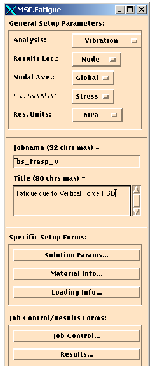
Now set the General Setup Parameters as follows:
1. Analysis: Vibration
2. Results Loc.: Node
The fatigue lives will be determined at the nodes of the model as with any other fatigue analysis.
3. Nodal Ave.: Global
Accept the default which means element contribution will be averaged as with any other fatigue analysis.
4. F.E. Results: Stress
Vibration fatigue uses S-N curves which require stresses; you do not have a choice.
5. Res. Units: MPa
Model dimensions are millimeters and forces are in Newtons, therefore stress units are MPa.
6. Jobname: bs_fresp_v
7. Title: Fatigue due to Vertical Force PSD
Solution Parameters
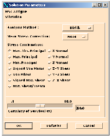
Open the Solution Params... form. Set the parameters as follows:
1. Analysis Method: Dirlik
The default is Dirlik which is the recommended method. If you select All, all the analysis methods mentioned in the theoretical background section will be used.
2. Mean Stress Correction: None
This is set to None in order to compare to the pseudo-static analyses which were also set to None. The mean stress correction is based on the same principles as that done for pseudo-static S-N fatigue analysis.
3. Stress Combination: Max. Abs. Principal
This is the default. In general this is the combination method that makes most sense. In actually, the ability to determine the principal stresses and their directions from the transfer function of stress components is a very unique feature of the vibration fatigue capability. Most FEA codes do not have this ability.
4. Certainty of Survival: 50%
This parameter is identical to that used in regular time based S-N analysis using the scatter in the S-N data to adjust the life prediction based on a probability of survival.
Click OK to proceed and close the form.
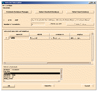
Material Information
Open the Material Info... form. This form is used to assign material and other information to regions of the model. In fact it is identical to the time domain S-N material set up form which you should be familiar with from previous exercises.
The Material Info... form and spreadsheet should then be filled in as follows:
1. Number of Materials: 1
2. Material: MANTEN
3. Finish: Polished
4. Treatment: No Treatment
5. Region: default_group
Accept the defaults for anything else on the form and close the form by clicking the OK button when finished.
Loading Information
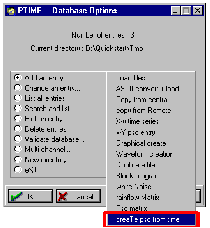
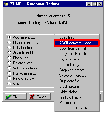
Open the Loading Info... form. Before completing this form we need loading input PSDs. These PSDs will be created from the time signals we used in the pseudo-static runs. On the Loading Info... form press the PSD Manager button. This will spawn PTIME, the loading database manager.
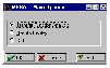
When PTIME appears, select Add an entry... | creaTe psd from time. This will spawn a utility module called MASD for creating auto spectral density functions. This module has multiple functions which are beyond the scope of this text. We wish only to create a Power Spectral Density function from a time series using MASD. A number of screens will be presented to you. Accept the defaults for all items except those indicated below:
1. Input Filename: 7d_44-50.dac
Click the OK button to accept this file and continue filling out the screen.
2. Output Type: Power Spectral Density
Click the OK button to proceed to the next screen.
3. FFT Buffer Size: 1024 : 0.9766 Hz width
This setting determines the number of points to define the PSD over the full frequency range. The full frequency range is from zero to 500 Hz which will give 1.024 pts/Hz or 512 points. Click the OK button to proceed to the next screen.
4. Output Filename: 7d_44-50
A file called 7d_44-50.psd will be created.
5. Plot Output: Yes
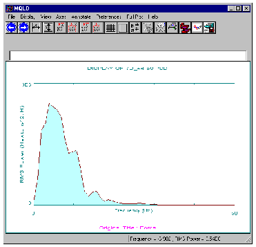
Click the OK button. The PSD will be created and a summary page will be shown. When this is closed the PSD will be plotted using the graphic module MQLD (quick look display).
6. View | Window X: Min=0, Max=50
To get a better look at the PSD, select the View | Window X menu pick and set the minimum frequency to 0 and the maximum frequency to 50. Use File | Exit to quit. This will return you to PTIME. Note the frequency content of this signal tapers off and is almost zero by 50 Hz.
7. Description1: Vertical Load
8. Number of fatigue equivalent units: 1
9. Fatigue equivalent units: Repeats
10. These last two inputs are ignored for a vibration fatigue analysis. But something must be supplied. All fatigue lives are reported back in seconds, hours or years.
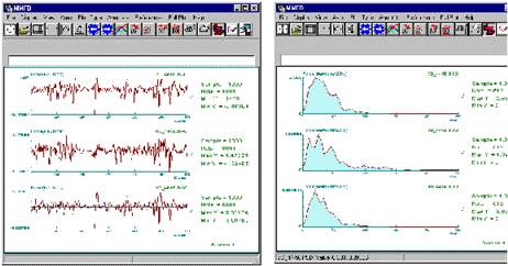
Repeat these steps for the other two time histories creating 8d_44-50.psd and 9d_44-50.psd for the horizontal and twist loads respectively. Then quit from PTIME. The original signals and their corresponding PSDs are shown below.
Hint: | PSDs can be created in a number of ways. They can be created as shown here from existing time signals. They can also be imported as ASCII text files (Add an entry... | ASCII convert + load) or they can be created manually by supplying xy points (Add an entry... | x-Y psd entry). |
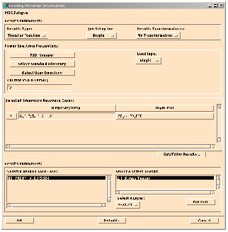
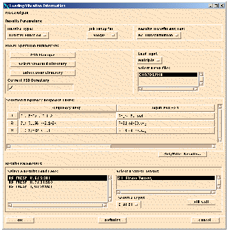
Once the PSDs are created you can proceed to fill out the appropriate information on the
Loading Info... form:
1. Results Type: Transfer hheader
The choice here is either Transfer Function or Power Spectrum. We are using transfer functions from FE analysis. It is also possible to calculate response PSDs directly in the FE analysis. In that case we would specify Power Spectrum. This will be covered later.
2. Results Transformation: Transform to Basic
This is the default setting. FE tensor results are transformed to the basic coordinate system to sum and average nodal contributions from adjacent elements. This must be done in a consistent coordinate frame. Unless you have a specific need we suggest you leave the default.
3. Load Input: Single
For this first example using the vertical loading PSD, we only have a single input. Multiple inputs will be covered later.
4. Frequency Resp: 6.(5-30)-2.1-2-
Clicking on the cell just below this title will activate a number of widgets on the bottom of the screen. This is where the Transfer Function from the FE analysis is selected. This is a multi-step operation so continue reading.
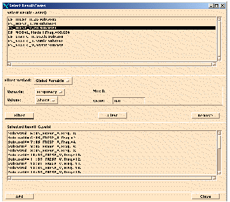
5. Get/Filter Results...
Open this form to select the Transfer Function of interest. You will see all Result Cases in the upper listbox. Select the BS_FRESP_V vertical Transfer Function Result Case. Click the Filter button. This will display all subcases (frequencies) associated with this Transfer Function in the lower listbox. If you click the Add button, the Result Case IDs will be transferred to the Loading Info... form listbox.
This form is quite versatile. You can remove various frequencies if you wish. You can filter based on various criteria. You can do multiple selections and fill the Loading Info... form listbox with multiple transfer function results (which will be necessary for a multiple input load analysis). It is suggested that you play with this form a bit to understand its usage. Press the Close button when you have successfully filled the listbox on the Loading Info... form with BS_FRESP_V,6.(5:30)- representing all the frequencies in the Transfer Function Result Case.
6. Select a Results Load Case: BS_FRESP_V,6.(5:30)-
Back on the Loading Info... form select this Result Case that you just filled in using the Get/Filter Results... mechanism. Once this is selected you will see the tensor results associated with this transfer function in the adjacent listbox.
7. Select a Stress Tensor: 2.1-Stress Tensor,
Select the only available tensor from this listbox. The layer information will update.
8. Select a layer: 2-At Z1,
This is displayed by default. Accept the default which is the top layer of stress of the shell elements.
9. Fill Cell
Click the Fill Cell button. This will fill the Frequency Resp. cell with the appropriate IDs in the spreadsheet above. The Input PSD cell then becomes active.
10. Select a PSD File Name: 7D_44-50.PSD
Select the PSD representing the vertical force which we created earlier.
The Loading Info... form is now complete. Click the OK button to accept the form. Before going on, however, a word or two on loading input PSDs is appropriate.
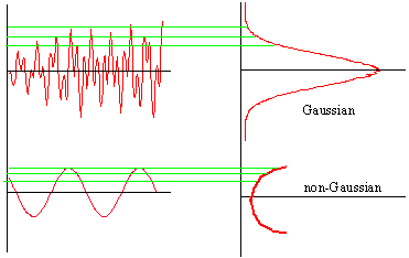
Vibration fatigue analysis makes certain assumptions of loading input. Those assumptions are that the signal is random, stationary and gaussian in nature. Random means that the signal contains no deterministically dominant event such as a spike occurring occasionally or a superimposed dominating sine wave. Truly random signals can only be characterized by their statistics such as root mean square (rms) and mean levels.
Stationary means that those statistics are not changing significantly with time. Any section of the signal should show very close statistical agreement.
Gaussian means that the peak and amplitude probability density function are gaussian in nature or follow a bell shaped curve as shown here. If you draw tram lines through a signal and count the number of times the signal passes through it and plot that as a density function it is gaussian if it follows a bell shape. An example of a non-gaussian signal is a pure sine wave. However adding multiple sine wave together quickly becomes gaussian.
Hint: | If you ever have the need to check the stationarity of a time signal, use the MSTATS utility module. MSTATS will give you running statistics of a signal and plot them for you. The increment of time history and overlaps can be specified. This is a very useful mechanism to determine stationarity. |
Job Control
Open the Job Control... form and set the Action to Full Analysis and click the Apply button to submit the job. Change the Action to Monitor Job and click the Apply button occasionally to monitor the job. This analysis will create the usual files: the job parameter file, bs_fresp_v.fin, the fatigue input file, bs_fresp_v.fes, and the fatigue results file, bs_fresp_v.fef. Also a message and status file are created (bs_fresp_v.msg, bs_fresp_v.sta). Unlike a standard time domain solution there is no intermediate rainflow count file, bs_fresp_v.fpp.
When the job is complete open the Results... form and with the Action set to Read Results, click the Apply button. This will read the results into the database for later viewing.
Additional Job Setups - Multiple Load Inputs
Now that you have seen how to set up the vertical load vibration analysis job you can repeat the setup procedures for the other two single input load (horizontal and twist loads). For the three single load input jobs you can follow the table below for Vibration analysis. Use default values if parameters are not specified.
Vertical Load | Horizontal Load | Twist Moment |
General Setup Parameters: |
Jobname: | bs_fresp_v | bs_fresp_h | bs_fresp_t |
Title: | Vertical Load | Horizontal Load | Twist Moment |
Solution Params Form: Analysis Method: Dirlik |
Mean Stress Correction: None |
Stress Combination: Max. Abs. Principal |
Design Criterion: 50% |
Materials Info Form: Material: MANTEN |
Finish: Polished |
Treatment: No Treatment |
Region: default_group |
Loading Info Form: Result Type: Transfer Function |
Load Input: Single |
Frequency Resp: | 6.(5.30)-2.1-2-
(BS_FRESP_V) | 7.(31-56)-2.1-2-
(BS_FRESP_H) | 8.(57-82)-2.1-2-
(BS_FRESP_T) |
Input PSD: | 7D_44-50.PSD | 8D_44-50.PSD | 9D_44-50.PSD |
Again, after each fatigue analysis is finished, read the results into the database under the Results form in the main MSC Fatigue form with the Action set to Read Results.
Correlated and Uncorrelated Loading
When each of these jobs is done we can now set up a multiple load input job with all three loads acting simultaneously. It is at this point however, that we have to decide whether the individual load inputs are correlated or uncorrelated. Simultaneously acting loads are said to be fully correlated if, in the time domain, the peaks and valleys from each signal occur simultaneously. This is normally the case for random load signals. Fully uncorrelated signals have the opposite true. Peaks and valleys do not occur at the same time and may cause a cancelling effect. Thus you would expect correlated loads to be more damaging than uncorrelated loads.
Since we are dealing with correlated loads, we need some way of determining the cross-correlation PSDs that will relate one input load PSD to another. If you have the original time series, this can be done with a MSC Fatigue module called MFRA (frequency response analysis). Start MFRA from a system prompt by typing mfra, or by selecting it from the Tools | Fatigue Utilities | Advanced Loading Utilities pull-down menu in Pre & Post or the Tools |MSC Fatigue | Advanced Loading Utilities pull-down menu in MSC Patran.
To get cross PSDs from MFRA follow these instructions after selecting Transfer Function Analysis from the main menu (use the defaults if not specified):
1. Input File: 7d_44-50.dac
Select the vertical load time history.
2. Response Filename: 8d_44-50.dac
Select the horizontal load time history. Click the OK button to accept these two file names.
3. Output Type: Power Spectral Density
Click the OK button to accept this screen and move to the next.
4. FFT Buffer Size: 1024 : 0.9766 Hz width
Select this buffer size so that there are the same number of points in the resulting cross-PSDs as in the PSDs created thus far. Click the OK button to accept this screen and go to the next.
5. Generic Output Filename: 7-8d_44-50
Give this cross term the name 7-8d_44_50 to indicate that the vertical load (7d) had been correlated with the horizontal load (8d).
6. Zero/Zero in Gain File: Zero
Click the OK button to proceed with the analysis.
Repeat this process to correlate 7d_44-50.dac with 9d_44-50.dac and 8d_44-50.dac with 9d_44-50.dac and use the output file names of 7-9d_44-50 and 8-9d_44-50 for the two respectively. Exit from MFRA when you are finished or you may plot the results using Results Display on the main menu of MFRA.
You will have in your directory three files called 7-8d_44-50.sxy, 7-9d_44-50.sxy and 8-9d_44-50.sxy. These are the cross PSD terms. Next, invoke PTIME and load these three new PSD files in using the Add an entry | Load file option so that they exist and are known in the PTIME database. Use a wild card to specify all three at the same time, i.e., *.sxy. Accept all defaults and click OK. Exit from PTIME when you are finished.
PSD Matrix File
One last step must be performed before the Loading Info... form can be properly filled for a multiple input load job. We must create a matrix file that relates the cross PSD terms with the input load PSDs. There are two ways to do this. Since we want to look at the effect of both uncorrelated loads and correlated loads we will introduce you to both methods by creating two matrix files.
Perhaps the easiest method is to manually create the file and then load it into PTIME. Create a file using any editor that looks like this in your working directory and call it cor789.pmx:
3
7d_44-50.psd 	7-8d_44-50.sxy 	7-9d_44-50.sxy
7-8d_44-50.sxy 	8d_44-50.psd 	8-9d_44-50.sxy
7-9d_44-50.sxy 	8-9d_44-50.sxy 	9d_44-50.psd
Note that the contents of this file are the names of the input load PSD files on the diagonal terms and the names of the cross PSD files on the off-diagonal terms. The first line indicates that there are three input loads and therefore the matrix is to be 3x3.
This file can be loaded into PTIME by using the option Add an entry | ASCII convert + load. Once in this option do the following:
1. ASCII Filename: cor789.pmx
2. Data Type: psd Matrix
3. PSD Matrix: cor789
Click the OK button to accept this screen and move to the next.
4. Description 1: correlated loads
Click the OK button to accept this screen and load the file.
The second method is a direct method within PTIME. Use the option Add an entry | Psd matrix. Follow these instructions:
1. Filename: uncor789.pmx
2. Description 1: uncorrelated loads
Click the OK button to accept this screen.
3. Enter Matrix Size: 3
Click the OK button to accept this screen. A spreadsheet will appear. In the diagonal cells of the spreadsheet type the names of the load input PSD files: 7d_44-50.psd, 8d_44-50.psd, and 9d_44-50.psd. Leave the other cells blank since this is meant to be uncorrelated. You must click the return or enter key for the file name to be accepted. Also the file must have been loaded into the PTIME database and physically exist. When you have filled out the spreadsheet select File | OK. This will load the new matrix file uncor789.pmx.
If you look at the contents of the second file it should look like this:
3
7d_44-50.psd 	NONE 	NONE
NONE 	8d_44-50.psd 	NONE
NONE 	NONE 	9d_44-50.psd
Loading Information - Multiple Load Inputs
Finally you can return to the Loading Info... form and set the job up for a multiple input load analysis.
1. Results Type: Transfer Function
2. Results Transformation: Transform to Basic
3. Load Input: Multiple
This will cause a listbox to appear with the PSD matrix files listed.
4. Select a PSD file: COR789.PMX
When you select the matrix file it will automatically update the spreadsheet on the form to indicate the number of input loads (number of rows). You must then supply a transfer function for each input load.
5. Frequency Resp:
6.(5-30)-2.1-2-
Clicking on the first cell just below this title will activate a number of widgets on the bottom of the screen. This is where the Transfer Functions from the FE analysis are selected. This is a multi-step operation.
6. Get/Filter Results...
Open this form to select the Transfer Functions of interest. This operation is identical to what you did for a single load input except this time you need to fill the listbox with all three Transfer Functions. Select the BS_FRESP_V vertical Transfer Function Result Case. Click the Filter button. This will display all subcases (frequencies) associated with this transfer function in the lower listbox. Click the Add button, the Result Case IDs will be transferred to the Loading Info... form listbox. Do the same for BS_FRESP_H, and BS_FRESP_T Transfer Function Result Cases clicking the Add button to add them to the listbox. Click the Close button when you have successfully filled the listbox on the Loading Info... form with BS_FRESP_V,6.(5:30)-, BS_FRESP_H,7.(31:56)-, and BS_FRESP_T,8.(57:82)-.
7. Select a Results Load Cases: BS_FRESP_V,6.(5:30)-
Back on the Loading Info... form select this Result Case that you just filled in using Get/Filter Results... mechanism. Once this is selected you will see the tensor results associated with this transfer function in the adjacent listbox.
8. Select a Stress Tensor: 2.1-Stress Tensor,
Select the only available tensor from this listbox. The layer information will update.
9. Select a layer: 2-At Z1,
This is displayed by default. Accept the default which is top layer of stress of the shell elements.
10. Fill Cell
Click the Fill Cell button. This will fill the Frequency Resp. cell with the appropriate IDs in the spreadsheet above. The next cell then becomes active so you can associate the next transfer function to its corresponding input load PSD. Repeat steps 7 through 10 for the horizontal and twist loads selecting the appropriate Transfer Function respectively.
Close down the Loading Info... form. Go to the General Setup Parameters and give the job the name bs_fresp_vth_c and the title correlated loads. Submit the job as you did for the single load input jobs and when the job is complete read the result into the database as done before.
Run one last job before investigating the results. Go into the Loading Info... form and change the matrix PSD file to UNCOR789.PMX. Give it the jobname bs_fresp_vth_u with the title uncorrelated loads and submit the job and read the result when finished.
Do not forget to read the results in from these two jobs.
Results
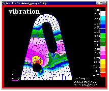
Perhaps the most obvious thing to do first is to make contour plots of fatigue life from the various jobs run so far. All of the fatigue analyses should have been run and the results imported into the database, so open the Results application switch on the main menu bar (remember not to confuse this with the Results... button on the main MSC Fatigue form).
When the Results application appears, make sure the Object is set to Quick Plot. You will see many Result Cases in the top listbox. Scroll all the way down to the bottom and select the Result Case that corresponds to the vibration fatigue analysis called Vibration Analysis, bs_fresp_vfef. Select Log of Life (Seconds) and click the Apply button to produce a plot. The plot is shown below.
Design Optimization
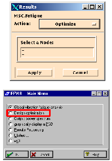
Let us now investigate the design optimization (sensitivity) capabilities of the vibration fatigue analysis. This is analogous to those capabilities in the S-N and strain-life analyzer FEFAT. The design optimization feature can be invoked directly from the Results... form with the Action set to
Optimize or from FEVIB started at the system prompt by typing
fevib and then entering the
Design optimization menu pick.
Do this with any of the vibration fatigue jobs completed thus far.
After specifying a jobname, if necessary, and selecting a node of interest and supplying a design life, the program will proceed to a summary report screen reporting the same life as the global analysis. When the summary report is closed you are placed in the main menu of the design optimization mode. The operation is identical to that of FEFAT’s design optimization mode and is therefore left to you to investigate its many options.
The only unique option to FEVIB’s design optimization mode is its ability to calculate life due to all the analysis methods (Dirlik, Narrow Band, etc.). This is done under Sensitivity analysis | Analysis methods (all).
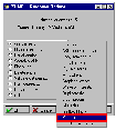
To see the statistical nature of the vibration analysis, you may want to plot the rainflow cycle count histogram, which is really a probability density function of rainflow ranges. In order to plot the histogram you will need to do the following from the Design Optimization main menu:
1. Select Original Parameters:
This will reset everything to the original parameters in case you have changed anything while investigating this tool.
2. Select Change Parameters:
Enter the Change Parameters screen and change the next two items below.
3. Mean Stress Correction: Goodman
4. Global Offset Stress: 0
Keep this set to zero. We must run a Dirlik plus mean stress correction in order to obtain a histogram plot. Click the OK button to return to the main menu.
5. Select Recalculate
6. Select results Display |plot Cycles histogram
This will plot the histogram. Change the view to 2D viewed from the left so you can see the stress ranges. This is done by selecting Plot-type | View Left.
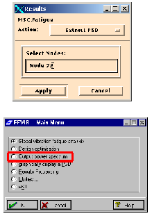
Stationarity Checks
As a last exercise before we go on to the second model of the bracket, let us look at another feature of the vibration fatigue analysis module FEVIB. Again invoke FEVIB from the system prompt and this time select the Output power spectrum option. Or on the Results... form set the Action to Extract PSD and click Apply.
Supply a jobname if necessary. The job we want to extract a PSD from is the multi-input correlated load case, bs_fresp_vth_c at Node 72. Do the following after supplying the proper jobname:
1. Generic Output Filename:
You can accept the default here. However, be aware that all file names created from this option will have the node number appended to the output filename.
2. Nodes/Elements to Select: 72
3. Combination Method: Abs Max principal
4. Interpolation Method: Linear
5. Stationarity Check Output: Yes
Be sure to turn this on. Press the OK button to continue. A result summary screen will be presented. Press the End button to continue.
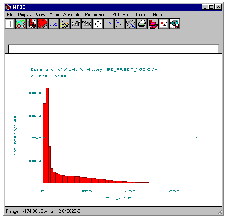
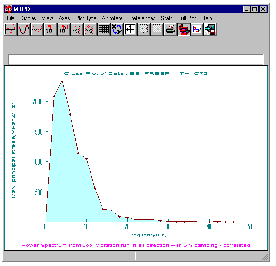
6. plot Power v. Frequency
At this point you are presented with three options for displaying different types of plots. Plot each one of them separately. The first is the stress response PSD as calculated by FEVIB at Node 72. This is, of course, calculated by multiplying the input PSD by the Transfer Function. For multiple inputs this becomes a matrix operation.
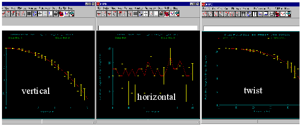
The second plot (angular deviation v. Load case) shows the total angular spread of the principal stress axes for each load case. The solid red line is plotted through the median value at each load case. The yellow error bars indicates the total deviation for each load case; the first load case being the first yellow error bar, the second, the second load case, and the third, the third load case, from left to right.
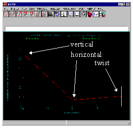
The third plot (angular deviation v Load Frequency) shows how the principal stress axes change with respect to frequency for each load case - actually three different plots.
The angle vs. frequency plot for the vertical load case shows a total angular deviation of the principal stress axes of only about two degrees according to the y-axis labels. The horizontal load case is very small, almost zero, and the twist shows a total of about 20 degrees. These corresponds to the single yellow error bars on the angle vs. load case plot for each load case. The yellow error bars on the angle vs. frequency plots indicate how the stress axes change due to differential damping at each frequency. In other words, it represents how the principal stress axes change subject to a sine wave load input at that frequency.
All angle spreads reported on these plots are relative to an arbitrarily selected angle. The angle vs. load case plot shows the angles relative to each other. You can see that there is about a 45 degree difference between the vertical load case and the horizontal and twist load cases, these two being very similar. This is as expected also in that the horizontal and twist loads are inducing a shear state at Node 72 whereas the vertical load case is not. This is confirmed by plotting the principal stress at Node 72 using the Results application.
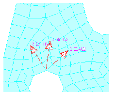
Hint: | To make these plots in Pre & Post or MSC Patran using the Results application, set the Object to Marker, the Method to Tensor, and select the appropriate Result Case. Show the tensor as 2D Principal and turn off the Min principal. It also may be desirable to only show the arrows and not the tensor box (under Display Attributes). The principals can also be animated to see the change in angle over frequency when all frequencies have been selected from a particular Transfer Function. The above plots were made from the static load cases. |
These angular spread plots are characteristics of the model. To see whether or not there may be a problem with stationarity of the principal stress axes, you must look at the regions of interest on the response PSD (between zero and 25 Hz) and the corresponding frequency locations on the stationarity plots. For all three load cases, there is little movement of the stress axes in this region.