XXXXXXXXXXXXXXXXXXXXXXXXXXXXXXXXXXXXXXXXXXXXXXXXXXXXXXXXXXXXXXXXXXXXXXXXXXXXXXXXXXXXXXXXXXXXXXXXXXXXXXXXXXXXXXXXXXXXXXXXXXXXXXXXXXXXXXXXXXXXXXXXXXXXXXXX''"> Problem 6: Spot Weld Analysis
H-Profile Spot Weld
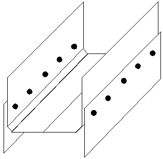
The following example is intended as an illustration of the spot weld method. The component is a laboratory test specimen made from a mild steel V-1147 with two rows of five spot welds. The test piece is illustrated in
Figure 14‑12. The specimen is loaded in tension so that the spot welds are subject to shear loadings. A series of constant amplitude tests were carried out with a load ratio (minimum to maximum load) of 0.1.
Note that the FE model is a half model due to the plane of symmetry. The model consists of two sheets of shell elements joined by five bar elements representing the spot weld nuggets. The bars are stiff and have a length equal to half the sum of the sheet thicknesses.
The spot weld fatigue analysis system was used to predict load-life curves for these test specimens. The calculation was based on the S-N curves for spot welds in (Ref. 32.) derived for spot welds in St1403 with thicknesses from 0.66 mm to 2.5 mm and spot weld nugget diameters from 3.5 mm to 6.5 mm.
Figure 14‑12 H-Profile Spot Welded Laboratory Specimen
This particular example assumes knowledge of the MSC.Fatigue job setup.
Step 1: Geometry and Results
The geometry and results are provided in the file called spotweld.op2 which can be found in the examples directory provided with MSC.Fatigue.
<install_dir>/mscfatigue_files/examples
Step 2: Material Characterization
The Material Info. form needs a bit more information than for other analysis types. Namely, there will be an S-N curve defined for each sheet that connect the spot welds as well as for the spotweld nugget itself. These are provided in the MSC.Fatigue materials database as spot_sheet_generic and spot_nugget_generic respectively. In addition, you must define the thickness of the sheets and the diameter of the spot weld nugget. There are also a number of other spot weld S-N curves defined in the materials database.
Step 3: Loading Histories
Define a time history with R=0.9 by entering XY points in PTIME using three points at 100, 1000, and 100 in a similar manner to previous problems. Call the load history name “spotweld.” The loading is Force, in Netwons.
Step 4: Setup MSC.Fatigue Job
Read in the old fatigue job setup. You will need the file called spotweld.fin. We will not actually run the fatigue analysis in this example as it is quite time consuming. Rather we will read in the job setup and discuss it briefly.
Operation | Comments |
patran | Invoke MSC.Patran (or MSC.Fatigue Pre & Post) if you have not already done so. |
File / New... | Open a new database from the File pull -down menu. Call it “spotweld.” Set the analysis preference to MSC.Nastran if asked. Ignore any warning messages. |
Analysis / Import | Open the Analysis application from the main form of MSC.Patran or the Import application in MSC.Fatigue Pre & Post. |
Action: Read Output2
Object: Both
Method: Translate | Set the Action, Object, and Method accordingly. |
Select Results File... | Select the result file spotweld.op2. Press the Apply button to import the model and static results. |
Group / Create... | Create a group with only the bar elements in it (the spot welds). These are elements 201, 202, 208, 209, and 210. Call the group “bars.” |
Tools / FATIGUE... (Analysis) | Invoke MSC.Patran’s FATIGUE interface by selecting it from under the Tools pull-down menu (or the Analysis application switch in MSC.Fatigue Pre & Post. |
Jobname: spotweld | Enter the jobname “spoweldt” and press the RETURN or ENTER key. This will read in the job parameters. Inspect the job setup forms to see how they are set up. |
Job Control... | Go to job control and click Apply with the Action set to Full Analysis and the job will run. |
Step 5: Evaluate Results
The results of the fatigue analysis can be read in using the appropriate option from the fatigue Results form.
The spot weld fatigue results can be postprocessed in a number of ways:
1. By listing the global results file.
2. By plotting the results in MSC.Patran. MSC.Patran’s Insight application is particularly good for this, allowing the fatigue life of each spot weld to be clearly visualized in the form of color coded spheres attached to each beam element.
3. Detailed information may also be obtained about the life, damage, stresses and forces at each calculation point (i.e. 108 sets of results per spot weld). Use the SPOTW module in interactive mode. Type spotw at the system prompt or invoke it from the Results or Job Control form.
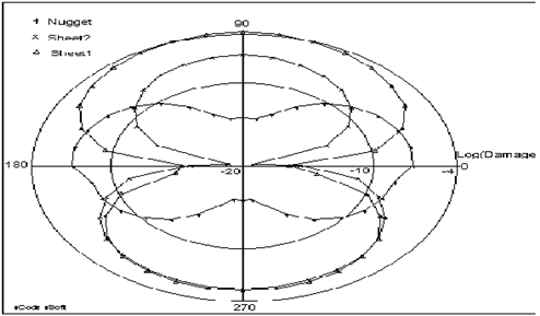
4. Damage may also be visualized in the form of a polar plot as in
Figure 14‑14. A polar plot shows damage at discrete points around the spot weld. There will be three curves on each plot corresponding to each location of the spot weld, i.e, the nugget and the two locations where the spot weld connects to the sheets. Use the module SPOTW in interactive mode.
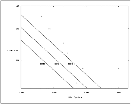
The studies so far indicate that in a typical application such as an automobile, the system correctly identifies all spot weld likely to give rise to durability problems. Using generic S-N curves as in this problem, life predictions tend to be conservative as shown in
Figure 14‑13. When S-N curves are used which are more representative of the material from which the component is constructed, more accurate life predictions can be made.
Figure 14‑13 Comparison of Test Data with Scatter Band
Figure 14‑14 Polar Plot of Damage in Most Damaged Spot Weld
T-Beam Specimen
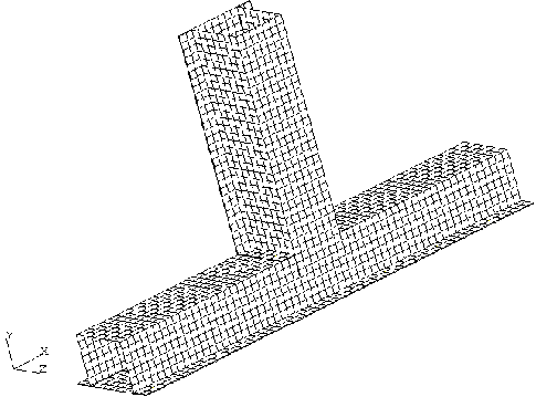
The second example concerns a spot welded T-piece. It is composed of sheets of thickness 1.0 and 0.8 mm. The finite element model of this structure is illustrated in
Figure 14‑15 below.
Figure 14‑15 Finite Element Model of T-beam Specimen
The T-beam specimen was clamped at the two ends of the cross-piece and could be loaded in either the x or z direction at the end of the vertical. The following cases have been tested and analyzed in the table below, once again using the generic spot-weld S-N curves.
Table 14‑13 Case | Experimental Life (cycles) | Predicted Life (cycles) |
F(x) amplitude 157.5 N R = 0.1 | 460,000 | ~500,000 |
F(z) amplitude 503 N R = -1 | 70,000 | ~35,020 |
F(z) amplitude 400 N R = -1 | 290,000 | ~145,500 |
Step 1: Geometry and Results
The geometry and results are provided in the files called t_beam_x.op2 and t_beam_z.op2 which can be found in the examples directory provided with MSC.Fatigue.
<install_dir>/mscfatigue_files/examples
Step 2: Material Characterization
The material is the same as defined in the previous spotweld example.
Step 3: Loading Histories
Define three time histories, one with R=0.1 and the other two with R=-1 with the appropriate amplitudes as in
Table 14‑13. This is most easily done by creating sine waves under the Wave Creation option with Max/Min values of 350/35, 503/-503, and 400/-400 respectively. Call the load history names “tbeam1,” “tbeam2” and “tbeam3” respectively.
Step 4: Setup MSC.Fatigue Job
Read in the old fatigue job setup. You will need the file called tbeam.fin. We will not actually run the fatigue analysis in this example as it is quite time consuming. Rather we will read in the job setup and discuss it briefly.
Operation | Comments |
patran | Invoke MSC.Patran (or MSC.Fatigue Pre & Post) if you have not already done so. |
File / New... | Open a new database from the File pull -down menu. Call it “spotweld.” Set the analysis preference to MSC.Nastran if asked. Ignore any warning messages. |
Analysis / Import | Open the Analysis application from the main form of MSC.Patran or the Import application in MSC.Fatigue Pre & Post. |
Action: Read Output2
Object: Both
Method: Translate | Set the Action, Object, and Method accordingly. |
Select Results File... | Select the result file t_beam_x.op2. Press the Apply button to import the model and static results. You can do the same for the other load case t_beam_z.op2, except import the results only. |
Group / Create... | Create three groups with only the bar elements in them (the spot welds). These groups should contain elements 3080:3095, 6267:6274, and 6237:6266. Call the groups “0.8_to_0.8,”, 0.8_to_1.1,”, “1.1_to_1.1”, respectively. |
Tools / FATIGUE... (Analysis) | Invoke MSC.Patran’s FATIGUE interface by selecting it from under the Tools pull-down menu (or the Analysis application switch in MSC.Fatigue Pre & Post. |
Jobname: tbeam | Enter the jobname “tbeam1” and press the RETURN or ENTER key. This will read in the job parameters. Inspect the job setup forms to see how they are set up. |
Job Control... | Go to job control and press Apply with the Action set to Full Analysis and the job will run. You can repeat this and the previous step for jobs “tbeam2” and “tbeam3.” |
Step 5: Evaluate Results
The results of the fatigue analysis can be read in using the appropriate option from the fatigue Results form as described in the previous spot weld example.
There appears to be reasonable correlation between the tests and the analysis, given the assumptions made. Clearly the predicted load-life curve is somewhat conservative compared to the experimental data, particularly for shorter lives. There are a number of possible reasons for this:
1. There may be a significant difference between the fatigue strength of spot welds in V-1147 and those in St1403 which were used to build the S-N curves used in the calculation.
2. A better spot welding technique may have been used in the specimens.
3. When the S-N data for shear loadings were processed(Ref. 32.), it seems that the effect of axial forces in the bar elements may have been neglected. In practice there is some axial force in shear tests which is quite sensitive to the geometry of the test assembly.
4. Because the forces and moments on each spot weld are based on FE calculations, S-N curves depend not only on the tests carried out to derive them, but also on the FE calculations used to obtain the forces. The same standard of FE modelling must be used in the S-N curve derivation and any subsequent life prediction. In particular it seems that changing the mesh density changes joint stiffness and the relative importance of the forces and bending moments on individual beams. More research is needed to establish best practical FE modelling techniques.
5. The failure criterion used in the test data plotted here was 30% decrease in stiffness. The failure criterion used to derive the basic S-N curve is not known.